Shortest Path on a Graph: Dijkstra and A* Algorithms

Table of Contents:

• Introduction to Graph Theory: Fundamentals and Applications
• How Dijkstra's Algorithm Works
• The History of Dijkstra's Algorithm: From Idea to Implementation
• Dijkstra's Algorithm in Python: Step-by-Step Implementation
• The A* Algorithm: Overview and Application
• An Efficient Python Implementation of the A* Algorithm
• Comparison of Dijkstra's and A* Algorithms: Which to Choose?

Introduction to Graph Theory: Fundamentals and Applications

Graph theory is a key field of mathematics and computer science devoted to the study of graphs, which consist of vertices and edges. Graphs play an important role in modeling systems and relationships found in real life. They are used in various fields, such as computer science, social media, transportation systems, and many others. Understanding graphs allows us to analyze complex structures and optimize processes, making graph theory an indispensable tool in modern research and technology.

Dijkstra's algorithm is an effective method for finding the shortest paths in graphs. It allows us to determine the minimum distance from one vertex to another, making it indispensable in fields such as navigation, transportation systems, and network analysis. Due to its versatility and speed, Dijkstra's algorithm is widely used in applications that require route optimization and cost minimization.

Graphs can be directed or undirected, depending on the nature of the connections between vertices. Graph edges can have weights that reflect the strength or cost of a connection. For example, in social network graphs, users are the vertices, and friendship connections are the edges. These connections can be measured by the frequency of message exchanges, allowing for analysis of network interactions. Graphs play an important role in various fields, such as data analysis, computer networks, and social research, providing efficient methods for representing and processing information about relationships.

The applications of graphs extend beyond social networks and span a wide range of fields. Graphs are actively used in computer science to analyze network structure, in transport logistics to optimize routes, and in bioinformatics to model interactions between biological molecules. In finance, graphs help identify relationships between assets, and in telecommunications, they help manage network nodes. Thus, graphs play a key role in solving complex problems in a wide variety of fields, providing efficient representation and processing of data.

• modeling web pages and their relationships on the Internet;
• designing road networks, where vertices represent streets and edges represent intersections;
• studying the interactions of genes, proteins, and molecules in bioinformatics;
• optimizing logistics routes for the delivery of goods;
• controlling the movement of robots in automated systems.

How Dijkstra's Algorithm Works

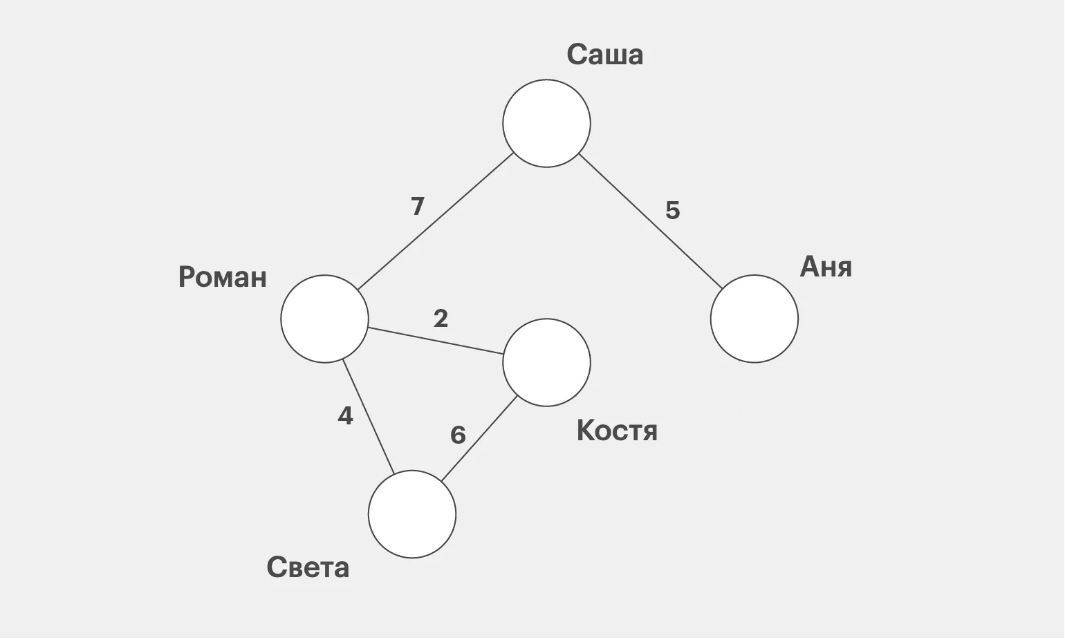
Dijkstra's algorithm is an effective method for finding the shortest paths in graphs. It allows you to quickly calculate the minimum distances from one vertex to another, which makes it indispensable in routing problems and in search engines. Using Dijkstra's algorithm significantly optimizes processes related to determining the shortest routes, which is especially important in areas such as transportation, telecommunications, and computer networks. This algorithm improves the efficiency and speed of data processing, which is relevant for modern technologies. In today's environment, where route planning has become an important part of everyday life, there are many ways to find the shortest route between cities, for example, A, B, C, D, E, and F. To determine the optimal route from city A to city C, you can use algorithms such as Dijkstra's algorithm or the A* algorithm. These methods allow you to effectively analyze the road network and find the minimum distance between two points. First, you need to create a map showing the distances between all cities. Then, you should apply one of the aforementioned algorithms, which will analyze possible routes, choosing the shortest path. It's important to consider not only distance but also potential obstacles, such as traffic jams or road closures, which can impact travel time. Using mapping services and navigation apps also greatly simplifies the task of finding the shortest route. These technologies can provide up-to-date traffic information and suggest optimal routes in real time. Thus, to quickly find the shortest route from city A to city C, it is necessary to use search algorithms and modern navigation tools, which will make the journey more convenient and efficient.

At first glance, the problem of choosing the shortest route between cities may seem simple: it is necessary to compare all possible routes, for example, A → B → C. However, as the number of cities (vertices) increases, the number of possible routes increases exponentially, making the problem significantly more complex. This phenomenon is associated with combinatorial explosion, when with each new vertex added, the number of combinations increases manifold. As a result, to effectively find the shortest path, it is necessary to use optimization algorithms and graph theory, such as Dijkstra's algorithm or the A* algorithm, which significantly reduce computation time and make it possible to find optimal routes even in complex networks.

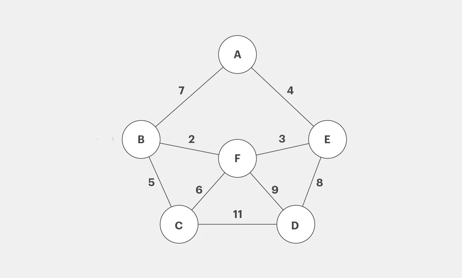
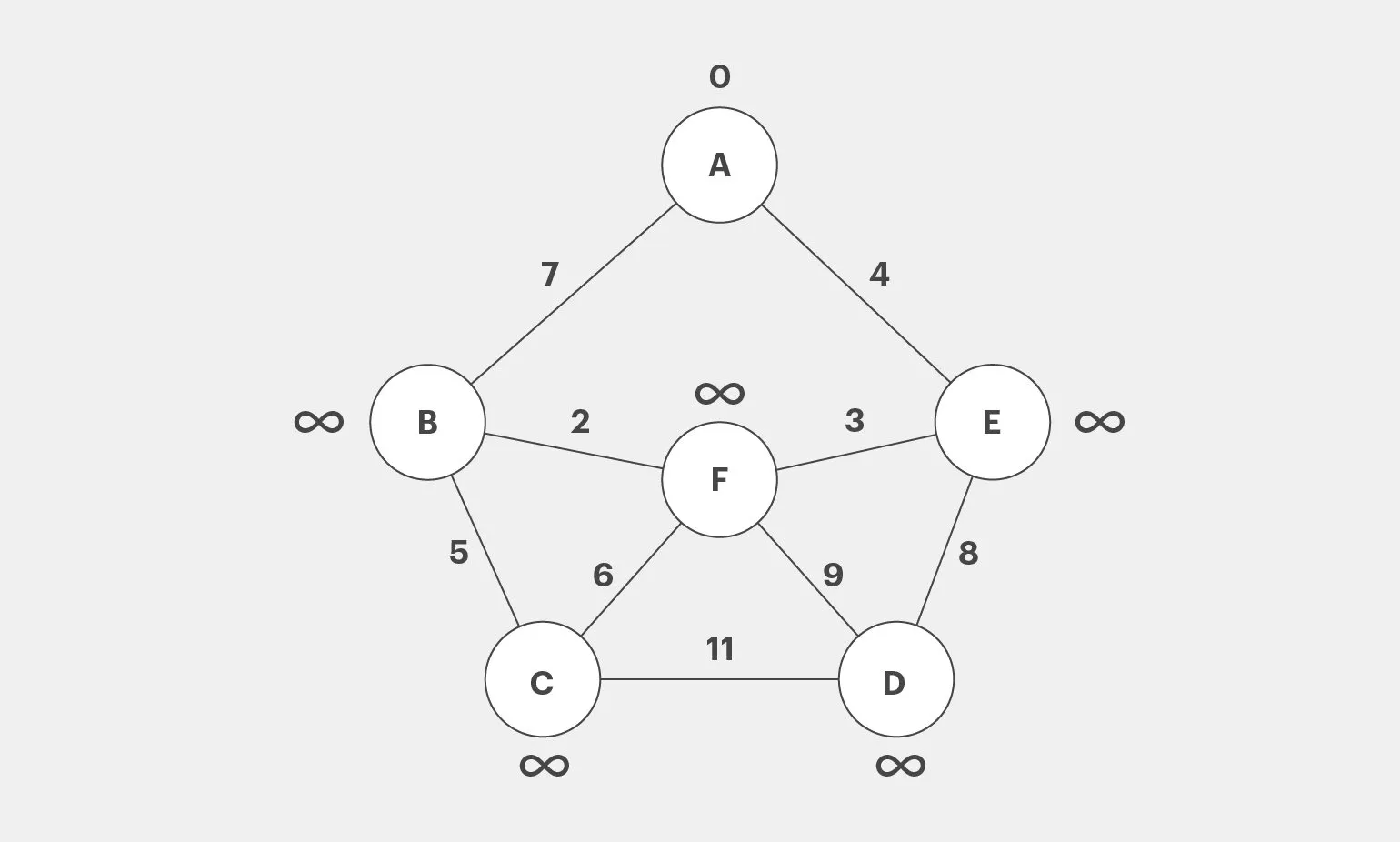
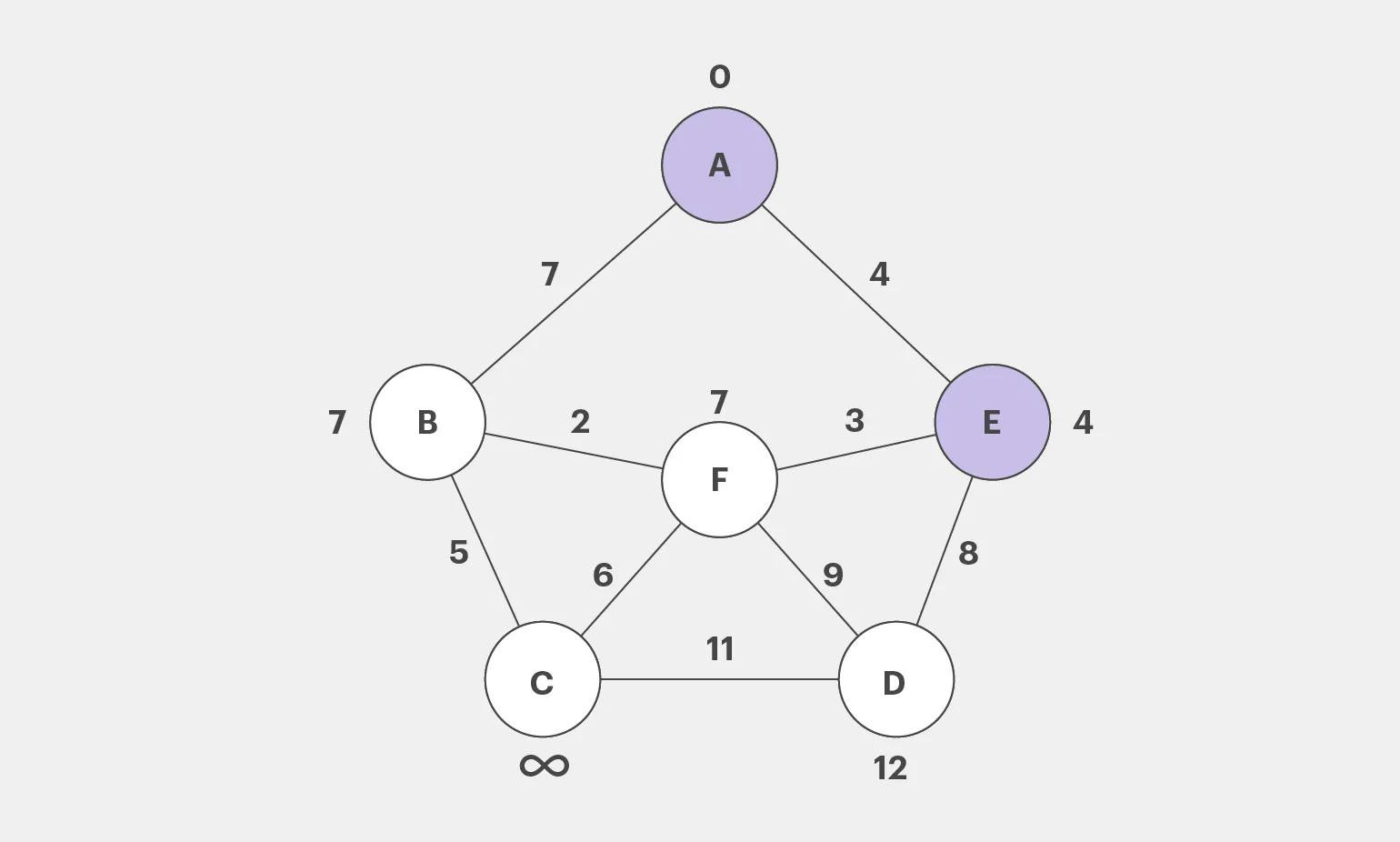
With more than 26 cities, even the most powerful supercomputer can require billions of years to enumerate all possible routes. In such situations, Dijkstra's algorithm comes to the rescue, effectively solving problems of finding the shortest path. This algorithm allows for a significant reduction in computation time by optimizing the process of finding the best route between cities. Dijkstra's algorithm is a key tool in graph theory and is widely used in various applications, including navigation systems and logistics. This algorithm doesn't simply enumerate all possible options; it uses a greedy approach. It sequentially selects vertices with the smallest distance, moving toward a given goal. This method significantly reduces computation time and ensures optimal results. The greedy algorithm is effective for shortest path problems, making it popular in a variety of fields, such as graph structures and routing. Let's return to our problem and start by determining the minimum distances from city A to all other cities: B, C, D, E, and F. This will allow us to better understand the relationship between these points and optimize routes for further calculations. In the first step, we will set the initial values ​​of the distances from vertex A. For vertex A itself, the distance will be 0, and for all other vertices, we will set the value to infinity, since we currently do not have data on the distances to them.

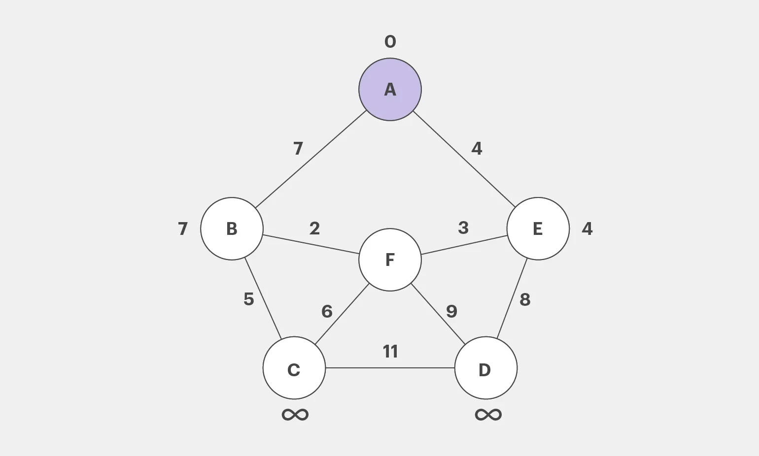
Let's consider the neighboring vertices of A, which are B and E, the distances to which are 7 and 4, respectively. Since these values ​​are less than infinity, we'll update them in our model. We'll mark vertex A as visited. This will allow us to more accurately estimate the path and continue analyzing the graph.

Now let's turn to the vertex with the minimum distance, then there is to E. Its neighbors, which have not yet been visited, are vertices F and D. Let's calculate the distances to these vertices:

• For F: 4 + 3 = 7
• For D: 4 + 8 = 12

Since the new values ​​are lower than the previous ones, they need to be updated. Vertex E will also be marked as visited.

The algorithm continues to select unvisited vertices with minimum values ​​and perform calculations until the shortest distance for each vertex is determined. This process ensures efficient finding of optimal paths in graphs, which is a key aspect in routing and network analysis problems.

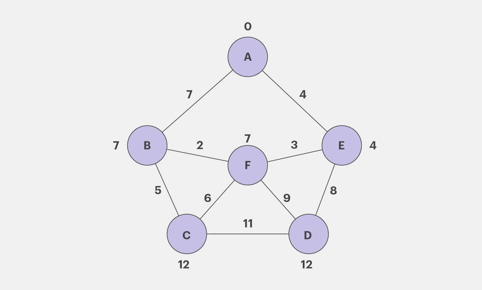
Our method can determine the shortest routes from point A to other cities. For example, we can find optimal paths that take into account various factors such as distance, travel time, and road conditions. This will allow for efficient trip planning and minimize transportation costs. Route optimization not only improves logistics but also increases travel convenience for users.

• From A to F: A — E — F
• From A to D: A — E — D
• From A to C: A — B — C

Dijkstra's algorithm has certain limitations. It can only be used for weighted graphs in which edge weights are known in advance. It is important to note that these weights must be non-negative. If the graph contains negative edge weights, Dijkstra's algorithm will not provide correct results. Therefore, when working with graphs that may contain negative weights, it is recommended to use alternative algorithms, such as the Bellman-Ford algorithm.

The History of Dijkstra's Algorithm: From Idea to Implementation

Dijkstra's algorithm, developed by the Dutch scientist Edsger Dijkstra in 1956, has become the basis for many modern applications in computer science and navigation. Dijkstra sought to demonstrate the capabilities of the new ARMAC computer and was looking for a problem that would be understandable even to those without prior computing experience. This algorithm effectively solves shortest path problems in graphs, making it an indispensable tool in a variety of fields, from geographic information systems to network protocol development. Dijkstra's algorithm remains relevant and in demand among specialists working with large volumes of data and complex network structures.

Edsger Dijkstra developed an algorithm for finding the shortest path, which became the basis for software used to plot routes on the Dutch transport map. This algorithm significantly simplified the travel planning process, marking a major advance in logistics and transportation. Its development made it possible to effectively find optimal routes, which positively impacted the quality of transportation services and improved travel management.

Dijkstra's algorithm was developed in a relaxed atmosphere. In an interview, Dijkstra shared a recollection of how, while having coffee with his fiancée on a café terrace in Amsterdam, he created an algorithm for finding the shortest path in twenty minutes. This algorithm was published three years later, in 1959. Dijkstra's algorithm has become the basis for many applications in route optimization and is an important tool in graph theory.

One of the reasons for the algorithm's elegance and efficiency is that it was developed mentally, without the use of paper and pencil. Dijkstra noted that one of the advantages of this approach is the desire to minimize complexity. This design method promotes clearer thinking and allows one to focus on the key aspects of the problem, which in turn leads to more optimal solutions.

Dijkstra's algorithm represents a significant achievement in the fields of mathematics and computer science. It was a key factor in Edsger Dijkstra's popularity as a scientist. Dijkstra himself noted that this algorithm became, to his surprise, one of the cornerstones of his fame. The algorithm is used to find the shortest path in graphs and finds application in various fields, including networks, transportation systems, and navigation applications. Its efficiency and simplicity have made it one of the most well-known and widely used algorithms in computer science.

For a more complete understanding of the algorithm and its practical applications, it is useful to study the materials on the GeeksforGeeks website and Wikipedia. These resources contain detailed explanations of Dijkstra's algorithm, its implementation using priority queues, and examples of its use in various problems. Familiarity with these materials will help better understand the basic principles of the algorithm and its effectiveness in finding shortest paths in graphs.

Dijkstra's algorithm continues to find application in various fields, such as navigation systems and network analysis, highlighting its versatility and importance in modern technology. This effective shortest-path finding technique allows for route optimization and improved service quality in areas such as transportation, telecommunications, and geographic information systems. Using Dijkstra's algorithm improves the accuracy and speed of data processing, making it an indispensable tool for developers and researchers.

Dijkstra's Algorithm in Python: Step-by-Step Implementation

Now that we've covered the theoretical foundations, let's move on to the practical part and develop code implementing Dijkstra's algorithm in Python. In this example, we'll determine the shortest distances from vertex A to all other vertices in the graph. Dijkstra's algorithm is an effective method for solving shortest path problems in graphs with non-negative edge weights. Let's create a function that takes a dictionary-formatted graph and a source vertex and then returns the shortest distances to all vertices.

For the algorithm to work efficiently, it's necessary to use the heapq module, which is part of the Python standard library. This module provides capabilities for working with heaps—a unique data structure in which the value of a parent node is always less than or equal to the values ​​of its children. This property of a heap allows for quick retrieval of the minimum element, making it useful for various algorithms, including sorting and implementing priority queues. Using heapq significantly optimizes insertion and deletion operations, which is especially important when processing large amounts of data.

Let's create a function dijkstra that takes two arguments: graph, representing our graph, and start, designating the starting vertex. This function will implement Dijkstra's algorithm for finding the shortest path from the starting vertex to all other vertices in the graph. Dijkstra's algorithm is effective for working with graphs where all edges have non-negative weights and allows you to find the minimum distances to each vertex. In the implementation of the function, we will use a priority queue to optimize the search.

Inside the function, we initialize the distances dictionary, which will store the distances from the starting vertex to all other vertices in the graph. We will also create a priority_queue heap for conveniently retrieving vertices with the smallest current distances. This will optimize the process of finding the shortest paths and improve the overall efficiency of the algorithm.

The algorithm will sequentially update the distances to neighboring vertices until it finds the shortest paths to all vertices in the graph. The results of the algorithm will be represented as a dictionary, in which the keys are the graph vertices, and the values ​​are the minimum distances from the starting point A to each of these vertices. This approach allows for efficient finding of shortest paths, which is an important aspect in problems related to graphs and route optimization.

Now we will calculate the shortest distances for our graph. For this, the graph will be represented in dictionary format, where the keys correspond to vertices, and the values ​​are dictionaries containing neighboring vertices and edge weights. This approach allows for efficient data processing and finding optimal paths between vertices, a key element in graph theory and search algorithms.

After creating the graph, call Dijkstra's function, passing it vertex A as the starting vertex. The result of the function will be displayed in the console. This approach allows for efficient finding of the shortest path from the starting vertex to other vertices in the graph.

We have successfully completed the implementation of Dijkstra's algorithm in Python. This algorithm finds shortest paths in graphs, making it an indispensable tool in route optimization problems. You can now use our code to solve various problems related to graph analysis and finding optimal routes. Using Dijkstra's algorithm opens up new possibilities for developing applications in navigation, logistics, and network analysis.

If you are interested in additional information and application examples of this algorithm, I recommend visiting resources such as GeeksforGeeks and Python.org. These sites offer extensive information and practical examples to help better understand the algorithm and its use in various scenarios.

The A* Algorithm: Overview and Application

The A* algorithm, pronounced "A star," is an effective tool for solving shortest-path problems. Developed in 1968, it has found wide application in fields such as robotics, navigation systems, and video game development. A* is an improved version of Dijkstra's algorithm, adding additional features that significantly increase the speed and efficiency of pathfinding. Due to its ability to take into account both the cost of movement and an estimate of the remaining distance to the goal, the A* algorithm provides optimal solutions in complex settings.

The A* algorithm is an efficient method for finding the optimal path from a starting point to a destination, similar to Dijkstra's algorithm. However, A* stands out because it combines two key components: the actual distance from the starting point and a heuristic distance estimate to the target point. The heuristic, in this case, is an approximate estimate that significantly speeds up the search process, making it more intelligent. Thanks to this combination, the A* algorithm provides faster optimal pathfinding in various applications, such as navigation systems and games.

To determine the shortest path between cities A and B, a heuristic function such as the Euclidean distance can be used. This distance is a straight line from the current point to the target point, allowing for a more efficient evaluation of possible routes. Using the Euclidean distance in pathfinding algorithms like A* significantly speeds up the process of finding the optimal route, as this estimate helps avoid unnecessary detours and directs the search toward the most promising options. Thus, the use of heuristic functions is a key element in route optimization problems.

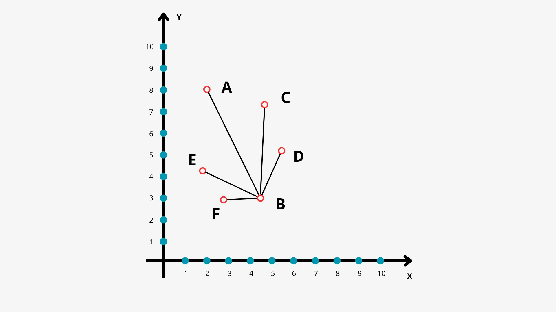
This graph displays heuristic distances from intermediate points to the final destination, ignoring existing road routes. This allows for a better understanding of the overall route structure and the evaluation of possible routes to reach the destination. The visualization helps identify optimal directions of travel and potential deviations from established routes, which can be useful for trip planning or transportation infrastructure analysis.

The Manhattan distance is one of the well-known heuristic functions used in various fields, including computer science and route optimization. The name of this function comes from the characteristic street system of New York City, where streets intersect at right angles. In such conditions, traveling between two points requires traveling parallel to the coordinate axes. This makes the Manhattan distance particularly suitable for evaluating routes in urban environments, where movement is often limited to straight lines. Using this heuristic allows us to effectively solve problems related to finding the shortest path and optimizing logistics in urban environments.

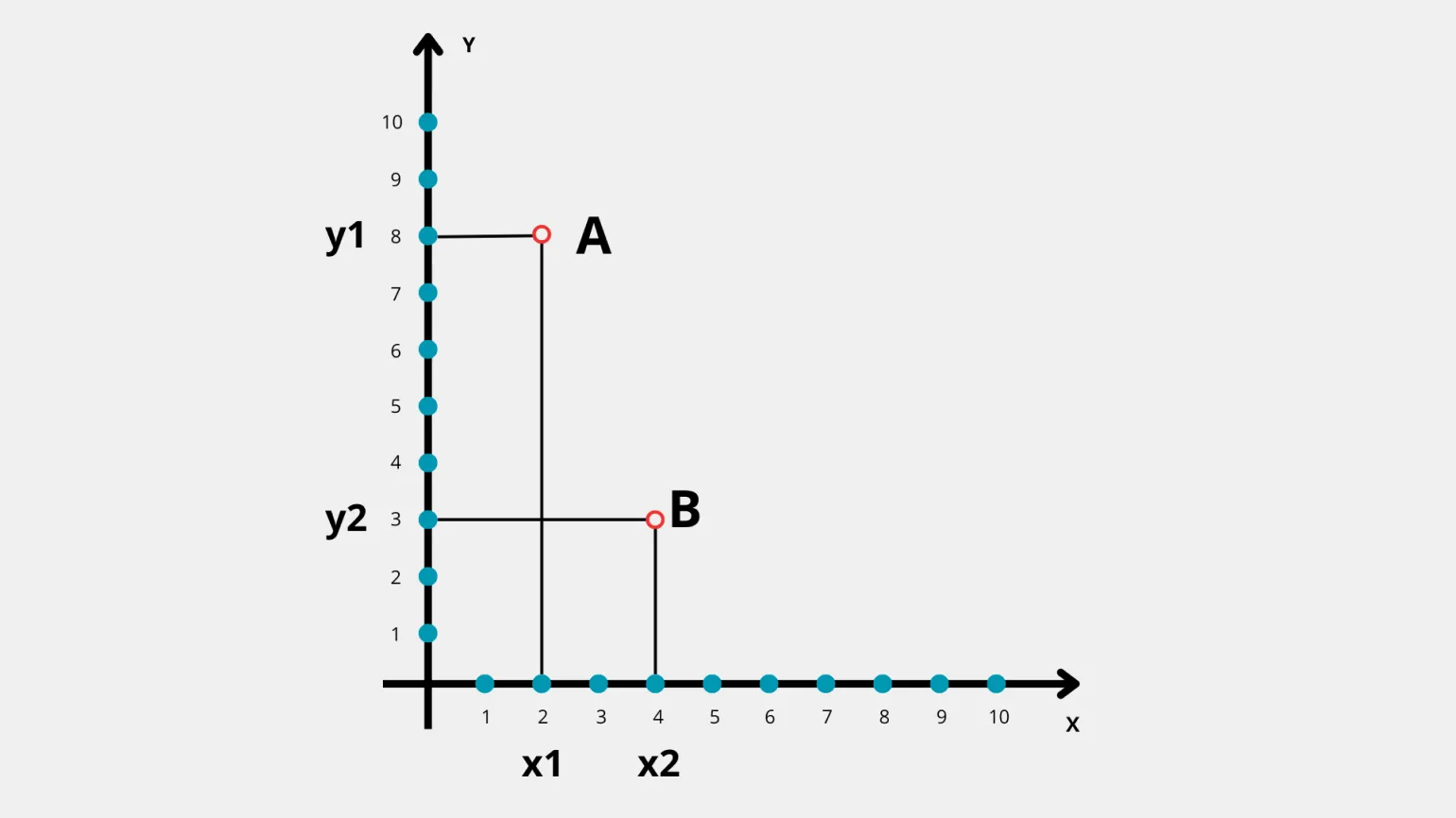
A simple formula is used to calculate the Manhattan distance between two points with coordinates (x1, y1) and (x2, y2). The Manhattan distance, also known as the urban distance, is defined as the sum of the absolute differences of their coordinates. The formula is as follows:

D = |x1 — x2| + |y1 — y2|.

This formula allows us to quickly estimate the distance between two points on a plane, moving only vertically and horizontally, which makes it especially useful in various fields such as logistics, robotics, and gaming. Understanding the Manhattan distance helps optimize routes and minimize costs when moving objects in urban areas.

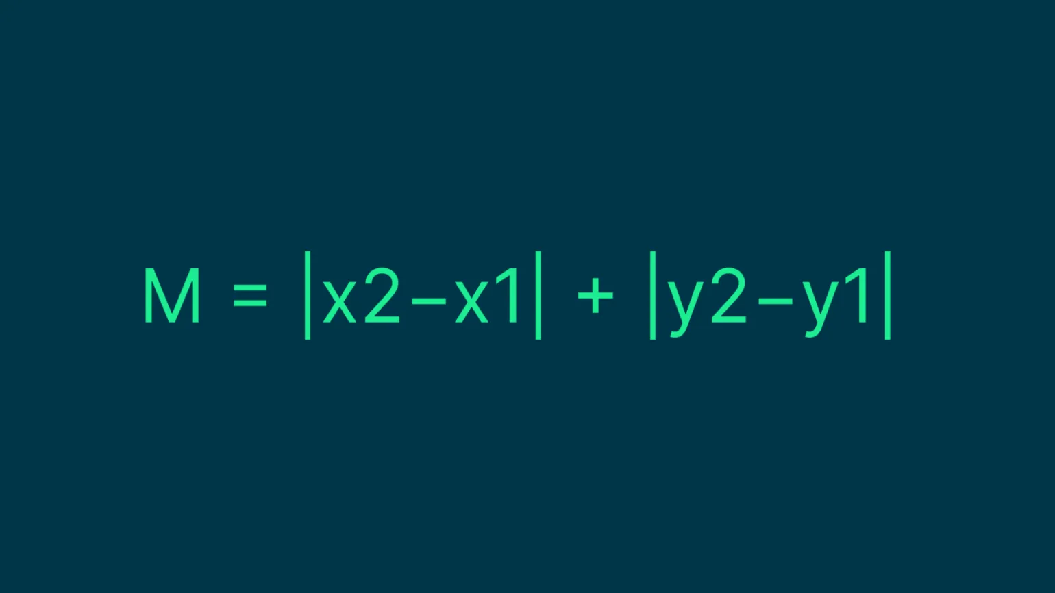
Let's look at an example of calculating the Manhattan distance. Let's say point A is at coordinates (2, 8), and point B is at coordinates (4, 3). Substituting these values ​​into the Manhattan distance formula, we get: M = |4−2| + |3−8| = 2 + 5 = 7. Thus, the Manhattan distance between points A and B is 7. This method is useful for analyzing distances in urban environments, where movement occurs on straight streets.

The A* algorithm is based on calculating two main values ​​for each vertex in a graph. The first value is the cost of the path from the starting vertex to the current one, and the second is an estimate of the remaining cost of the path from the current vertex to the goal. The algorithm combines properties of breadth-first search and greedy search, allowing it to efficiently find the shortest path. A* also uses a heuristic function that helps estimate the distance to the goal, significantly speeding up the search process. A* is used in various fields, such as route planning, games, and robotics, due to its ability to find optimal solutions in minimal time.

• g(n) is the length of the path from the starting vertex to the current vertex n.
• h(n) is a heuristic estimate of the distance from the current vertex n to the goal.

The A* algorithm selects the vertex with the minimum sum of g(n) + h(n) at each stage, carefully examining neighboring vertices. This process continues until the final goal is reached. Modern research confirms that the A* algorithm continues to be one of the most effective solutions for real-time pathfinding problems. Its applications span various fields, including robotics, game development, and routing, making it an indispensable tool for search optimization and efficiency.

An Efficient Implementation of the A* Algorithm in Python

Let's consider an implementation of the A* algorithm in Python using the Manhattan distance as a heuristic. The A* algorithm is an efficient method for finding shortest paths in graphs, making it particularly useful on two-dimensional grids. In this article, we discuss key aspects of the algorithm and provide an example implementation in Python. Using the Manhattan distance allows for efficient distance estimation to the goal, significantly speeding up the search process. The A* algorithm combines the advantages of Dijkstra's algorithm and greedy methods, making it an optimal choice for pathfinding problems.

The A* algorithm is an efficient pathfinding method that combines the actual distance from the starting point to the current one with a heuristic distance estimate to the goal. In this context, the manhattan_distance function is used to calculate the Manhattan distance between two points on the grid. This approach allows the A* algorithm to find optimal routes in various problems, such as navigation in games or route planning in robotics. By taking into account both real and estimated distances, the A* algorithm provides a faster and more accurate solution than other search methods.

The main steps of the A* algorithm implementation include the following elements:

The first step is to initialize the start and target points, where the coordinates and values ​​\u200b\u200bneeded by the algorithm are determined. Next, it is necessary to create two lists: an open one, which will contain the nodes to be evaluated, and a closed one, which will contain the tested nodes.

Then the main loop of the algorithm begins, in which the node with the lowest cost is selected from the open list. This node is evaluated for the presence of neighbors that can become part of the path. For each neighbor, the values ​​\u200b\u200bf f, g, and h are calculated, where f is the total cost of the path, g is the cost from the start point to the current node, and h is the estimated cost of the path from the current node to the target point.

If the neighbor has not yet been added to the open list, it is added to it. If it is already on this list, the g values ​​\u200b\u200bare compared, and the path is updated if necessary. After processing all neighbors, the current node is moved to the closed list.

The process continues until the open list is empty or until the target node is found. If the target is found, the algorithm returns the found path, which is optimal according to the given criteria.

Thus, the A* algorithm efficiently finds the shortest path in graphs using a combination of heuristics and cost estimates.

Defining a 5×5 grid, where obstacles are represented by units, is the first step in creating a shortest-path system. Next, it is necessary to implement a path recovery function that will track the optimal route from point A to point B. After that, the A* algorithm can be run, which searches for the best path given the given obstacles, and the results can be displayed. This process will provide an efficient solution to the navigation problem in a limited space.

After running this algorithm, you will get the optimal route from point A to point B. This is the final result of the code, which provides the shortest path.

This example illustrates the effective application of the A* algorithm to find the optimal route on a grid, using the Manhattan distance as a heuristic. The A* algorithm is a powerful tool for solving navigation and routing problems, allowing you to find the best paths in a variety of applications, from mobile maps to robotics. Using the Manhattan distance helps significantly speed up the search process, providing faster and more accurate results.

For more detailed information and code examples, we recommend referring to the official Python documentation at https://docs.python.org/3/. It is also useful to explore resources dedicated to algorithms, for example, information about the A* algorithm at https://www.geeksforgeeks.org/a-star-search-algorithm/. These resources will help you deepen your knowledge and better understand the application of various algorithms and libraries in Python.

Comparing Dijkstra's Algorithm vs. A*: Which One to Choose?

When choosing between Dijkstra's and A*'s algorithms for finding the shortest path, you should consider the specifics of the specific problem and the available data. Each of these algorithms has unique advantages and disadvantages. The optimal application of each depends on the context in which they are used, as well as the requirements for performance and search accuracy. Dijkstra's algorithm is well suited for problems that require finding the shortest path in equal-weight graphs, while A* is more efficient at solving problems with a heuristic approach, allowing you to find optimal solutions faster in large and complex graphs.

The key differences between these two approaches deserve a more detailed analysis. Both strategies have their own unique characteristics that can significantly affect the results. It is important to consider not only their advantages but also their disadvantages in order to make an informed choice. Let's consider how each approach affects efficiency and results, as well as what factors should be taken into account when making a decision.

• Dijkstra's algorithm is designed to find the shortest path from a single starting vertex to all other vertices in a graph. In contrast, the A* algorithm focuses on finding the shortest path to a specific goal, using a heuristic function to estimate the distance.
• One of the main differences is that Dijkstra's algorithm treats all vertices as equal and chooses the one with the shortest distance from the starting vertex. The A* algorithm, on the other hand, uses a heuristic function, which makes it faster and more efficient, especially in large and complex graphs.
• Dijkstra's algorithm may be less efficient on large graphs because it processes all possible vertices, which increases the execution time. The A* algorithm significantly speeds up the search process due to its ability to ignore less promising paths.

Dijkstra's algorithm is an excellent choice for finding the shortest paths from one vertex to all others in graphs, especially when heuristic information is lacking. Its effectiveness is demonstrated in situations where a robust and accurate solution is required. At the same time, if heuristic information is available that can speed up the search process, the A* algorithm significantly improves performance and allows for faster finding of optimal paths. The choice between the algorithms depends on the specific conditions of the problem and the available data.

When choosing between Dijkstra's algorithm and A*, it is important to consider the specifics of the problem, the size of the graph, and the availability of heuristic information. Dijkstra's algorithm is ideal for finding the shortest path in graphs with equal edge weights, while A* is more effective in situations where heuristics are available, allowing for faster solution search. For a more in-depth study and application of these algorithms, it's worth turning to resources like GeeksforGeeks and Wikipedia, which offer detailed explanations, examples, and practical tips.