Excel: 5 Features That Will Make Your Work Easier

Contents:

• CONCATENATE function: Efficiently combine data from multiple cells
• How a drop-down list in Excel speeds up table filling
• Pivot tables: Optimizing work with data for effective analysis
• VLOOKUP function in Excel: Simplifying work with data from different tables
• Logical functions in Excel: Checking values ​​and combining formulas
• Advanced Excel features: What is worth learning
• Learn Excel on Skillbox and become an expert

CONCATENATE Function: Efficiently Combine Data from Multiple Cells

The CONCATENATE function in Excel is a powerful tool for combining data from different cells into one. It offers more than just simple string concatenation, allowing users to separate information with spaces, commas, or any other characters of their choice. This function greatly simplifies working with data, making it more structured and easier to understand. Using the CONCATENATE function allows you to effectively organize data and create more informative reports and tables.

The CONCATENATE function is useful in a variety of situations. It allows you to collect product characteristics located in different cells into a single sentence. You can also use this function to combine last names, first names, middle names, phone numbers, and addresses of employees. The advantage of using a function is that data is combined without losing information. This is especially important when working with large tables containing a large number of rows. Using CONCATENATE, you can effectively organize and structure information, making it easier to analyze and work with.

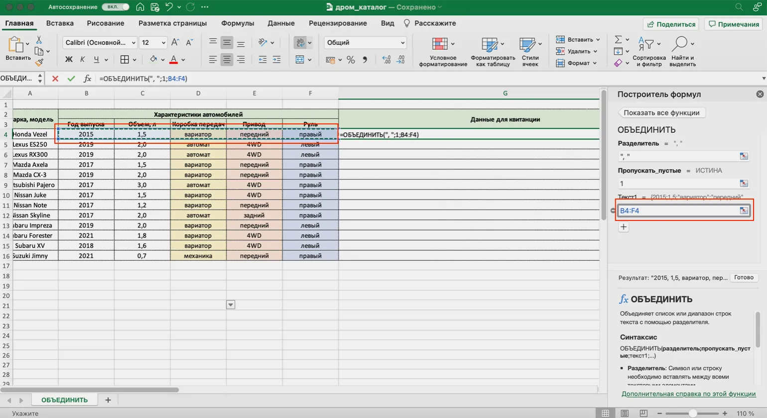
To use the CONCATENATE function, follow these simple steps. First, select the cell where the combined values ​​will be collected. Then, open the function builder and find the CONCATENATE function. Enter the required arguments, including the separator and the range of values ​​you want to combine. This function allows you to effectively combine text strings, which can be useful for creating reports or summarizing data in tables.

If you need to combine data from the range B4:F4, separating the values ​​with a comma and a space, use the formula: =CONCATENATE(«, «; 1, B4:F4). This formula will provide a compact and structured presentation of your data, making it easier to analyze and understand. Combining data in this way allows you to effectively organize information and make it more readable.

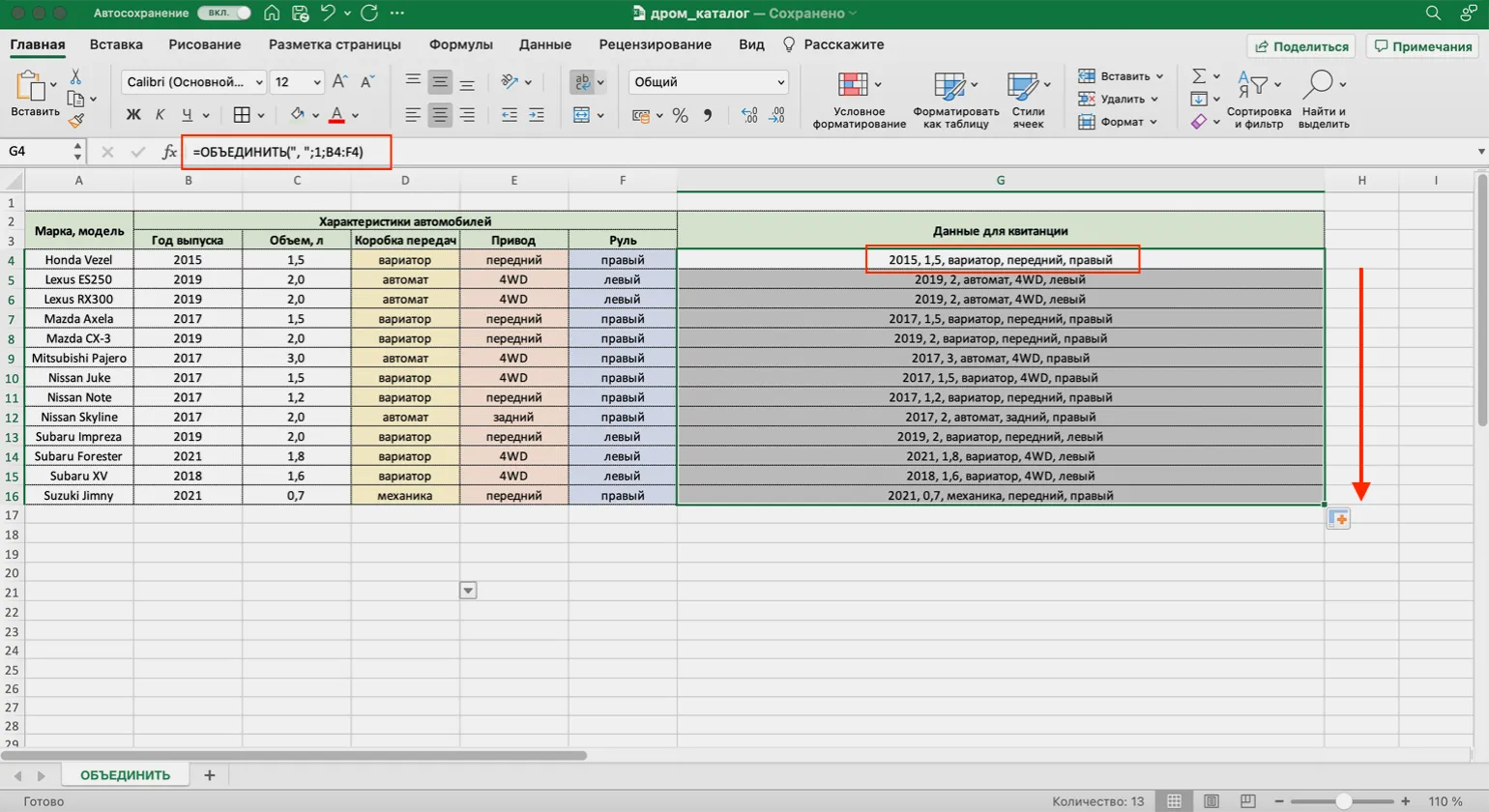
Ignoring the CONCATENATE function can result in manual data collection, which involves copying information from one cell and pasting it into another. While this approach may be acceptable for small spreadsheets, with thousands of rows, this work becomes tedious and time-consuming. Using the CONCATENATE function not only simplifies data processing but also significantly improves the efficiency of working with large volumes of information. Proper use of this function allows you to optimize your work with spreadsheets and avoid errors associated with manual data entry.

If you want to learn more about the CONCATENATE function, we recommend visiting the article on the Skillbox Media website. Here you will find useful tips and practical examples of using this feature, which will help you effectively apply it in your projects.

How a drop-down list in Excel speeds up table filling

A drop-down list in Excel is an effective tool for speeding up the entry of repetitive data. It allows users to quickly select values ​​from a predefined list, which significantly increases the productivity of working with tables. Using drop-down lists in Excel not only simplifies the data entry process but also minimizes the likelihood of errors associated with manual entry of information. This functionality is especially useful when working with large volumes of data where consistency and accuracy are required. Drop-down lists allow you to easily manage data, ensuring its structure and ease of further analysis.

A drop-down list should be used in cases where repeated entry of the same parameters is required, such as employee names or product names in a catalog. This significantly saves time and reduces the likelihood of errors, which helps maintain the consistency and correctness of data. Using drop-down lists improves the user experience and makes the process of entering information more efficient, especially in large forms and databases.

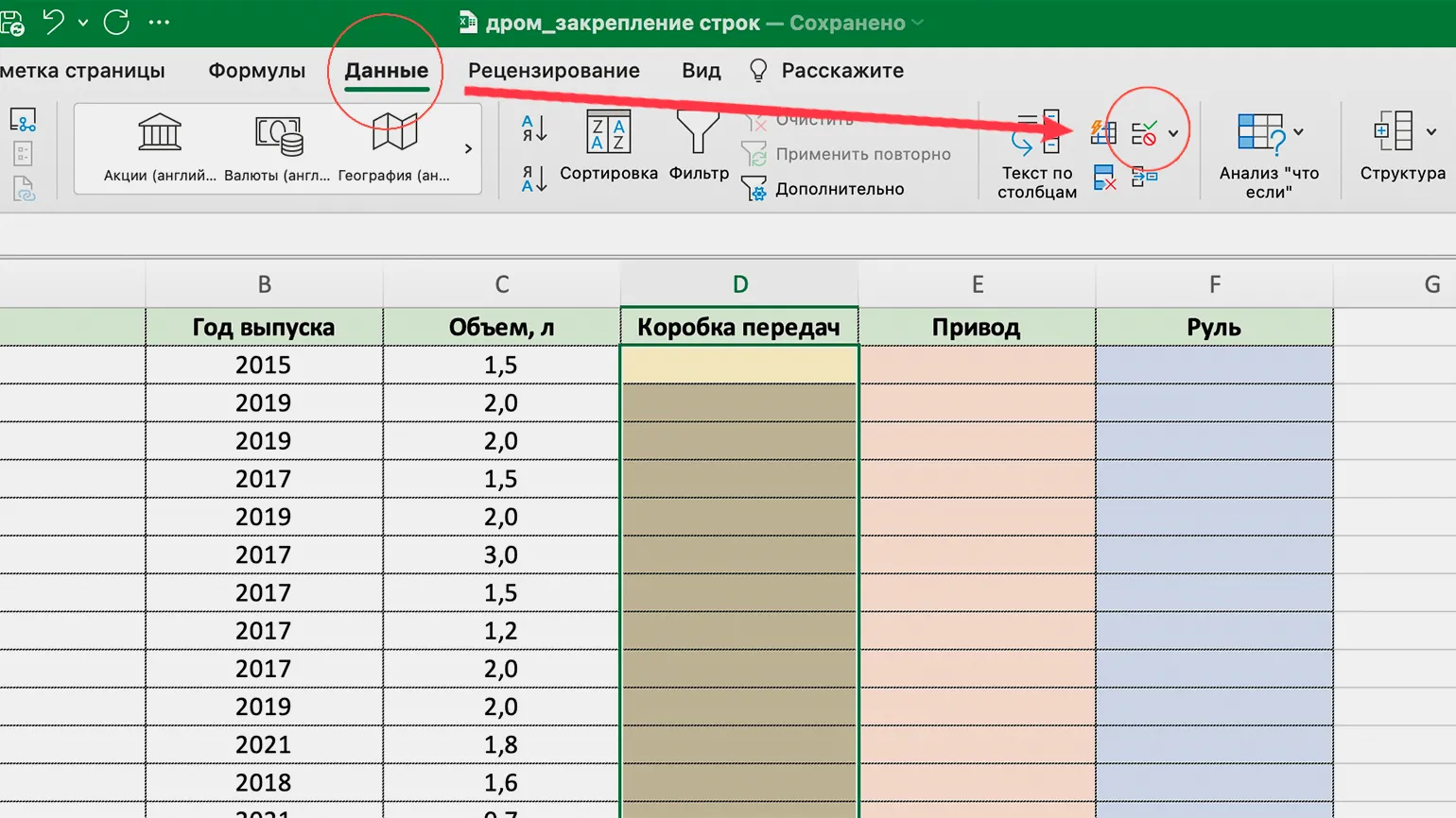
To create a drop-down list in Excel, follow these steps:

First, select the cell where you want to place the drop-down list. Then, go to the Data tab in the top menu. In the Data Tools group, click the Data Validation button. In the window that opens, select the Options tab. In the Data Type field, select List. In the Source field, Enter the values ​​for your drop-down list, separating them with commas, or specify the range of cells containing these values. Then click "OK." The drop-down list will now be available in the selected cell, making data entry easier and minimizing errors.

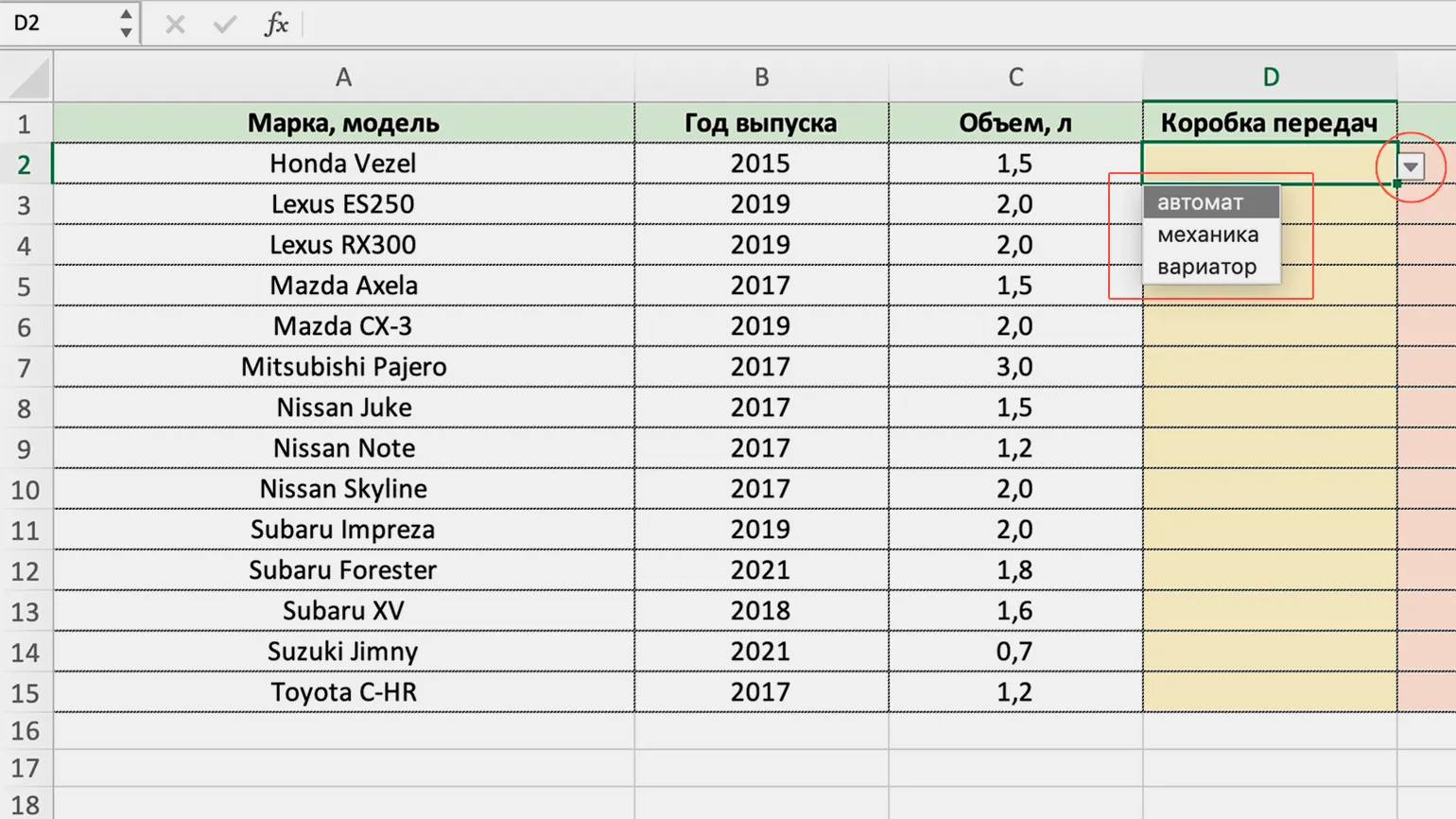
In the window that opens, select "Options," then click "Enable," and then select "List." Place the cursor in the "Source" field and specify the range of values ​​from the previous sheet. Then click "OK," and your drop-down list will be successfully created and ready for use.

Not using drop-down lists can lead to entering the same data multiple times, which increases the likelihood of errors. This is especially risky in situations where your attention is distracted and you begin to enter information carelessly. To avoid such problems and improve entry accuracy, we recommend using drop-down lists. This will not only simplify the process, but also make it more efficient and secure.

Save this guide from Skillbox Media to simplify the process of creating drop-down lists and increase the efficiency of working with data in Excel. This instruction will help you streamline tasks and improve the organization of information in your tables.

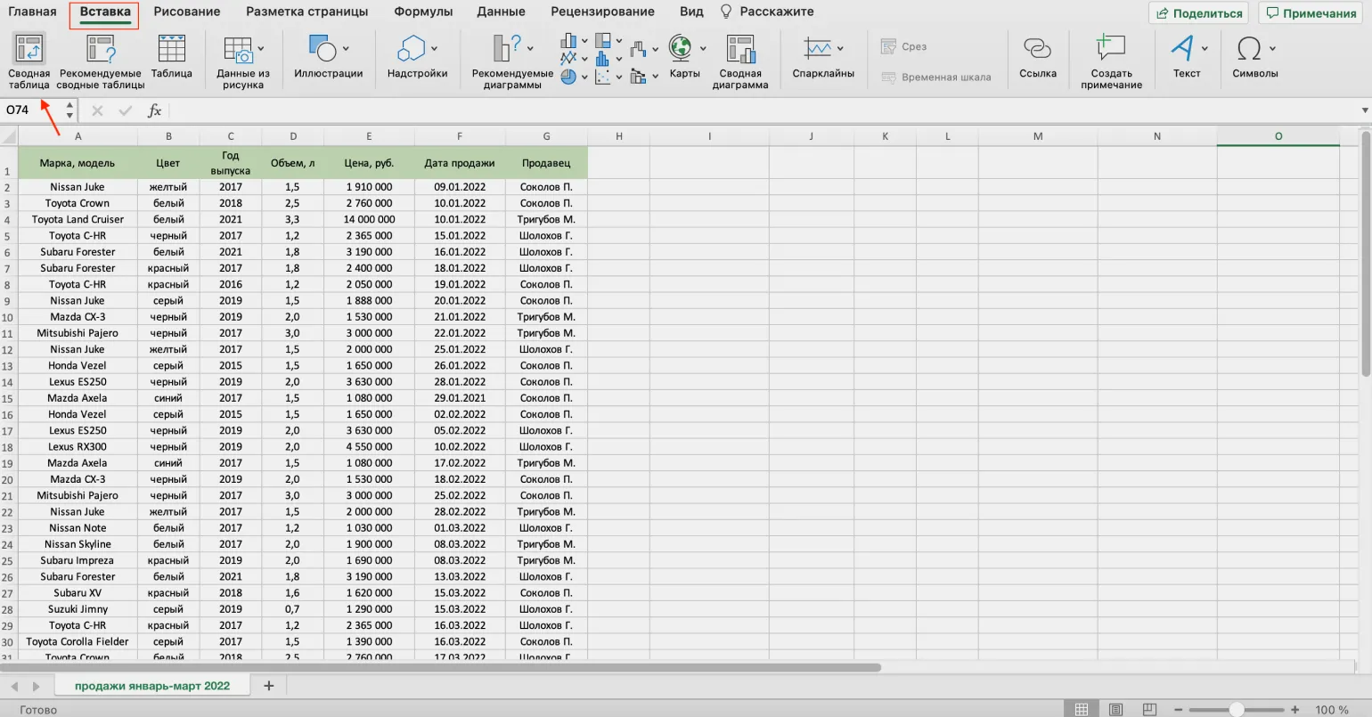
Pivot tables: Optimizing work with data for effective analysis

Pivot tables are an effective tool for analyzing and visualizing large amounts of data in Excel. They allow you to quickly aggregate information from various sources, process it, group it, and present it in visual reports that meet specific user needs. Using pivot tables simplifies working with data and promotes a deeper understanding of analytical information.

A pivot table is an indispensable tool for creating clear and structured reports based on disparate data. It is especially useful when you need to consolidate information on the performance of different departments, group employees by various criteria, and analyze their effectiveness. Using pivot tables, you can quickly extract useful insights and visualize data, allowing you to make informed decisions based on factual information. This tool helps not only in analyzing current performance but also in planning future actions to improve the organization's performance.

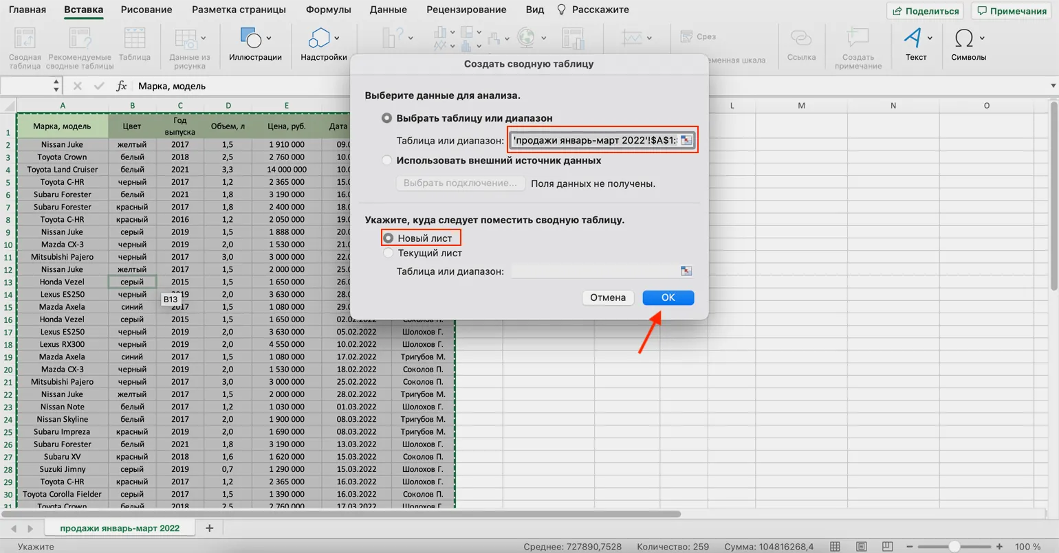
Creating a pivot table in Excel is a simple and intuitive process. Start by going to the "Insert" tab and selecting the "Pivot Table" button. In the window that appears, you need to specify two main parameters: the data range for analysis and the location where you want to place the new pivot table. Pivot tables allow you to quickly summarize, analyze, and visualize large amounts of data, making it much easier to work with. Choosing the right options at the outset will help you get the most accurate and informative results.

• The data range in the source table that will be used for the pivot table;
• The sheet to which the pivot table will transfer the processed data for further analysis.

After completing these steps, Excel will automatically create a new sheet for your pivot table. On the left, you will find the area designed to display the pivot table, and on the right is the PivotTable Fields pane. Here you can configure the necessary options to effectively organize and analyze your data. Setting up a pivot table will allow you to quickly obtain the information you need and visualize data in a convenient format.

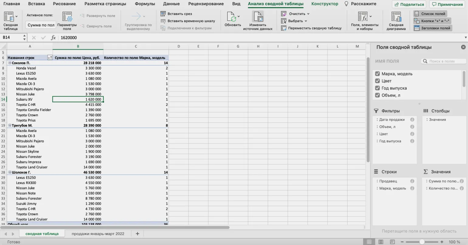
We've prepared a detailed step-by-step guide to help you gain a deeper understanding of the settings panel, filters, and calculations in a pivot table. This guide will be a valuable resource for anyone looking to improve their data skills and streamline their data analysis processes.

Ignoring pivot tables can lead to significant data processing difficulties. This will require you to manually process large volumes of information, perform complex calculations, and create reports, which will require significant time and effort. As data volumes increase, this work can become virtually impossible. Pivot tables simplify and automate this process, providing quick access to the information you need and allowing you to focus on analyzing data rather than manipulating it.

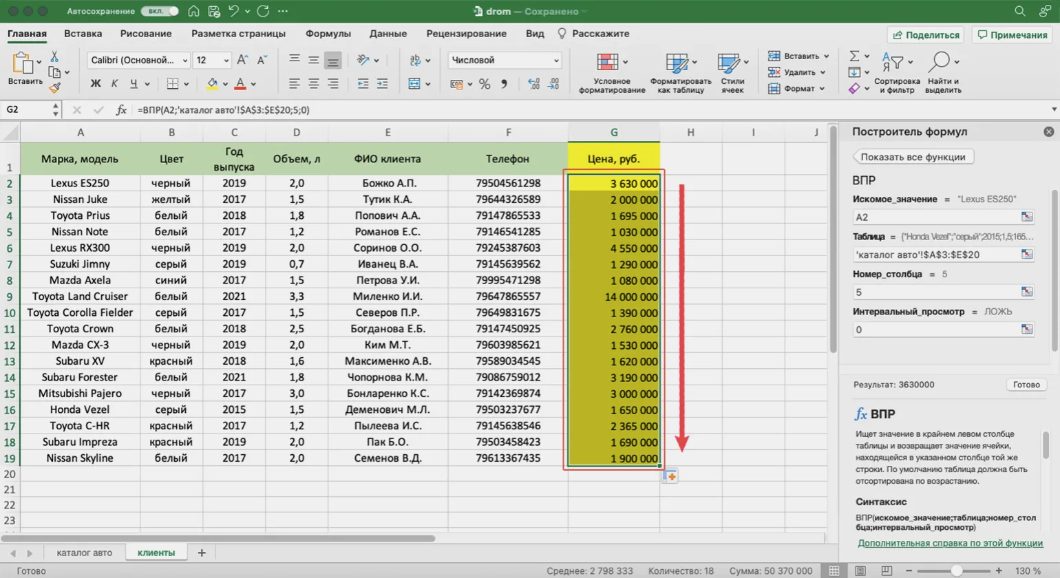
VLOOKUP Function in Excel: Simplify Working with Data from Different Tables

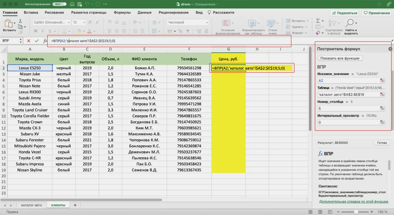
The VLOOKUP (Vertical Lookup) function in Excel is used to find data in one table and move it to another. It is especially effective when the data is not sequentially organized. With this function, users can quickly find the values ​​they need, greatly simplifying working with large amounts of information and increasing productivity. VLOOKUP allows you to search across columns, making it an indispensable tool for data analysis and reporting in Excel.

Using the VLOOKUP function becomes essential when you need to combine data from different sources. For example, you might want to create a separate table with employee salaries using information from the company's general register. You can also transfer product prices from a catalog to a sales table, facilitating data management and analysis. This function allows you to efficiently work with large volumes of information, ensuring convenience and accuracy in data processing.

Correctly using the VLOOKUP function in Excel requires several steps. First, select the cell that will display the value you want to look up. Then, go to the "Formulas" section and select "Insert Function." In the window that opens, find the VLOOKUP function. This function allows you to look up a value in the first column of a specified range and return a value from a specified column in the same row. Make sure all function parameters, including the search range and column number, are specified correctly to achieve an accurate result. Using the VLOOKUP function can significantly simplify data processing and increase the efficiency of working with tables.

• The lookup value is a cell with matching data in both tables where the function will perform the search.
• Table is the range of cells in which the function will search for values. It is important that this range includes both the columns with the lookup value and the column with the data to be transferred. The lookup value must be in the first column of the range.
• Column number is the ordinal number of the column in the source table where the value to be transferred is located. Numbering starts with 1 for the leftmost column.
• Range lookup is an option that determines the level of search precision. For an exact match, enter 0, and for an approximate match, enter 1.

After entering all the required parameters, click the "Done" button. The lookup value will be displayed in the specified cell. You can then drag the formula down to automatically fill in the remaining cells. This will allow you to quickly and efficiently process data in the table, saving time and increasing the accuracy of calculations.

If you don't use the VLOOKUP function, you'll have to search for the required data yourself and transfer it to another table. In this case, you'll have to go through the entire list of employees to find the relevant records and copy their salaries into your table. This will require a lot of time and effort, which can lead to errors and inaccuracies. Using the VLOOKUP function significantly simplifies the process of searching and processing data, allowing you to quickly and efficiently extract the necessary information.

For an in-depth study of the VLOOKUP function and its application in Excel, I recommend visiting the Skillbox Media website. There you will find detailed instructions, examples, and tips to help you effectively use this function in your projects.

Logical functions in Excel: checking values ​​and combining formulas

Logical functions in Excel are key tools for automating data analysis. They allow you to check whether specified conditions meet the criteria set in a specific range of cells. The result of these functions is a logical value: true or false, depending on whether the conditions are met. Using logical functions such as IF, AND, OR, and NOT significantly simplifies data processing and helps make informed decisions based on analysis. These functions are especially useful when working with large volumes of information, allowing you to quickly identify patterns and anomalies. Correct use of logical functions helps improve the efficiency of working with tables and improves the quality of data analysis.

Logical functions should be used in situations where it is necessary to analyze data and draw conclusions based on certain conditions. For example, when working with large product catalogs, you can quickly determine the availability of products in the price range of 14,000 to 25,000 rubles. This not only simplifies the data analysis process but also promotes faster decision-making, which is especially important in a competitive market. Using logical functions allows you to effectively manage your inventory and optimize business processes.

Logical functions in Excel play an important role when combined with other functions. For example, combining the VLOOKUP function with the IF logical function allows you to search by multiple criteria simultaneously. This significantly expands the possibilities of data analysis and makes it possible to combine several formulas in one expression. Using such combinations makes working with data more efficient and informative, allowing users to obtain accurate results and make informed decisions based on analysis.

This Skillbox Media article provides comprehensive information about Excel's logical functions. You'll learn practical examples of using the TRUE, FALSE, AND, OR, NOT, IF, IFERROR, ISERROR, and ISBLANK functions. These powerful tools will significantly improve your data skills and streamline your data analysis processes in Excel. Learning logical functions opens up new opportunities for automating calculations and increasing your work efficiency.

Ignoring logical functions can waste significant time, as you have to manually check each condition. This is especially costly when working with large volumes of data. Using logical functions helps automate processes and significantly improves analysis efficiency, allowing you to quickly process and interpret data without having to delve into routine work. Using these functions not only saves time but also reduces the likelihood of errors, making analysis more accurate and reliable.

Advanced Excel Features: What's Worth Learning

Excel is not only a spreadsheet tool but also a powerful platform for data analysis, modeling, and process automation. This application offers a variety of advanced features that allow you to effectively process and analyze large volumes of information. Discover the power of Excel and learn how its tools can simplify complex tasks and increase your productivity.

Arrays are data structures consisting of multiple adjacent cells that can be processed as a single unit. Using arrays can significantly speed up calculations. Instead of processing each cell individually, you can create formulas that perform multiple operations simultaneously. This significantly reduces the time required to solve problems, from hours to seconds. Optimizing calculations using arrays not only increases efficiency but also simplifies working with large volumes of data, which is especially important in today's information overload. Macros in Excel are an effective tool for automating processes, allowing you to record and play back sequences of actions with a single command. They are especially useful for performing routine tasks where repeating the same steps can increase the likelihood of errors. Using macros, you can significantly reduce the time required to perform repetitive operations, increase your productivity, and reduce the risk of errors. This makes macros an indispensable tool for users seeking to optimize their work in Excel. Power Query and Power Pivot are powerful tools for working with big data in Excel. They allow you to efficiently process and analyze significant volumes of information by loading data from various sources, such as ERP systems, web pages, and PDF documents. These add-ins have no row limit, allowing you to work with data exceeding Excel's 1,048,000 row limit without impacting performance. Using Power Query and Power Pivot significantly simplifies and improves data analysis, allowing users to focus on gaining important insights and making informed decisions. The advantages of using Power Query and Power Pivot include their high efficiency in processing large volumes of data, making these tools essential for analysis and modeling. They allow you to easily transform data into a workable format and create databases, significantly simplifying the process of analyzing information. Using Power Query and Power Pivot allows you to optimize workflows, improve data quality, and accelerate analytical results. These tools are ideal for professionals looking to improve their productivity and accuracy in working with data.

Learn Excel with Skillbox and become an expert

Skillbox offers a unique program, "Excel from Zero to PRO," suitable for both beginners wanting to master the basics of working with spreadsheets and professionals seeking to deepen their knowledge and skills in Excel. This course covers all essential aspects of working with Excel, including formulas, functions, creating charts, and working with large volumes of data. The training is conducted in a convenient format, allowing each participant to learn at their own pace and apply the acquired knowledge in practice. The program is aimed at developing practical skills that will help improve work efficiency and career prospects.

The course is taught by a team of experienced specialists: certified MS Office trainer Renat Shagabutdinov and Evgeny Namokonov, co-author of the book "Google Sheets: It's Easy." Their professional experience and practical knowledge will allow you to deeply master the program and achieve a high level of mastery in using Google Sheets. Gain valuable skills that will help you effectively work with data and improve your productivity.

During this course, students will acquire essential skills that will help them in their professional careers. They will learn to analyze information, develop strategies, and apply modern technologies in their work. Additionally, participants will gain experience working in a team, which will help develop communication skills and the ability to collaborate with colleagues. Each student will be able to create a portfolio reflecting the acquired knowledge and skills, which will increase their competitiveness in the labor market.

• Efficient execution of complex calculations using formulas and all necessary functions;
• Data visualization: sorting, filtering, creating charts and pivot tables;
• Forecasting: working with data arrays and calculating results in various scenarios;
• Integration with external data sources: import, export and transform information using Power Query and Power Pivot;
• Process automation: setting up macros and creating custom functions to solve unique problems.

Each student has the opportunity to complete homework assignments, which are analyzed by experienced experts. Course participants also have access to ready-made templates and cheat sheets, which significantly facilitates working with Excel. These resources help students better understand the material and improve their preparation for practical tasks.