
Contents:

Excel and Google Sheets: A Free Course for Beginners
Learn MoreHow to Freeze Rows in a Table
Freezing rows in a table is an important feature that allows users to always see the column headings, even when Scrolling down data. This is especially useful when working with large amounts of information, as it helps maintain context and facilitates data analysis. In this article, we'll take a detailed look at how to freeze the top row or rows in a table, making your work more efficient and organized. Learn how to use this feature to streamline your workflow and increase your productivity.
- Select any cell in your table.
- Click the View tab.
- On the toolbar, select Window and then Freeze Top Row.
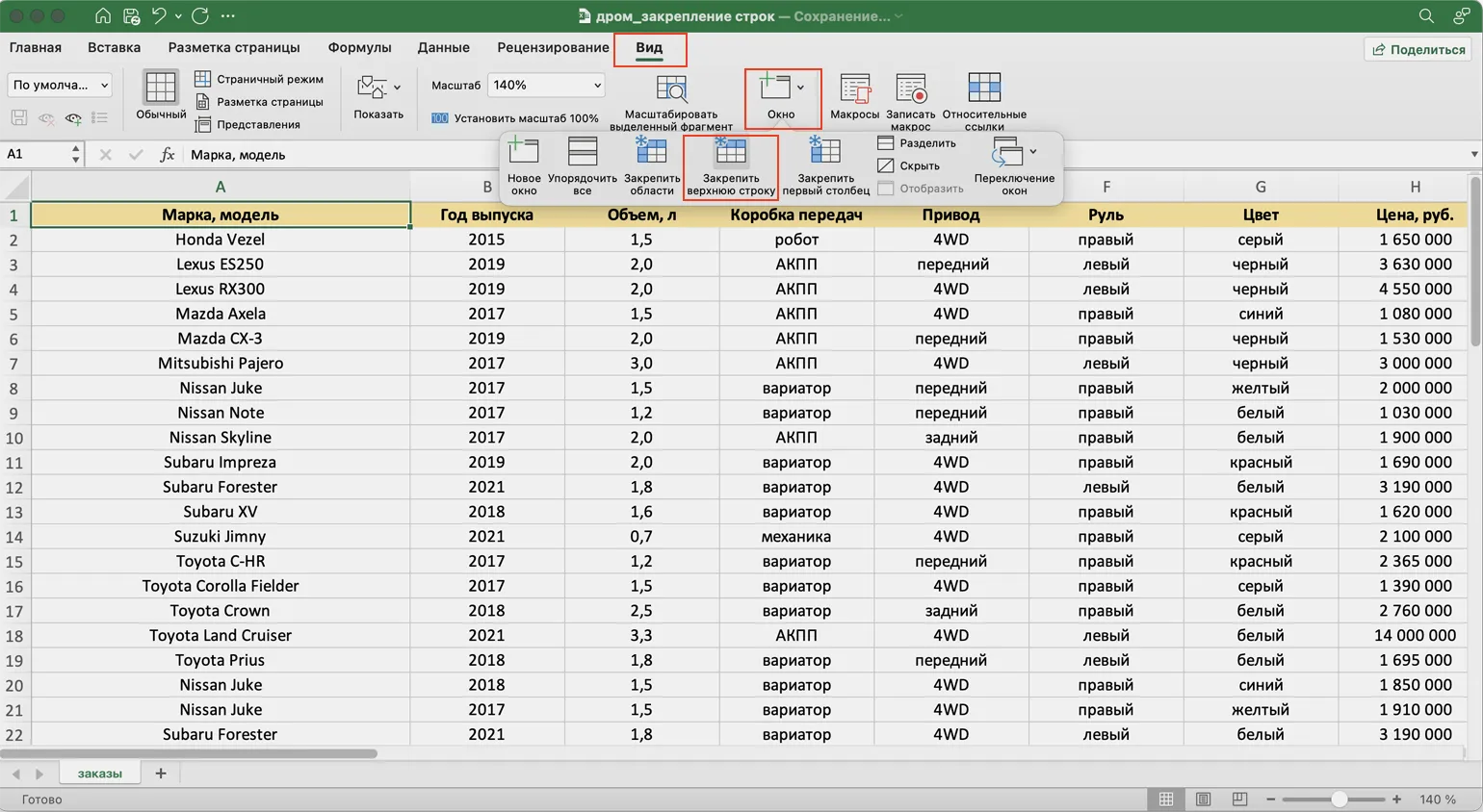
After completing these steps, a border will appear under the first row, ensuring the column headings are visible from anywhere on the sheet. This is especially effective when working with long tables, allowing the user to easily navigate the data and improving the perception of information.
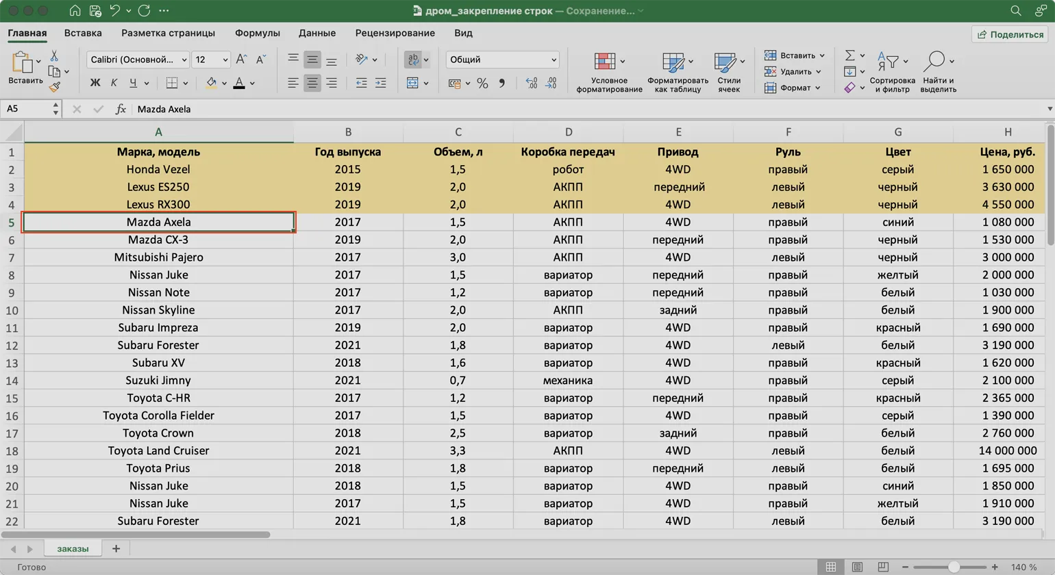
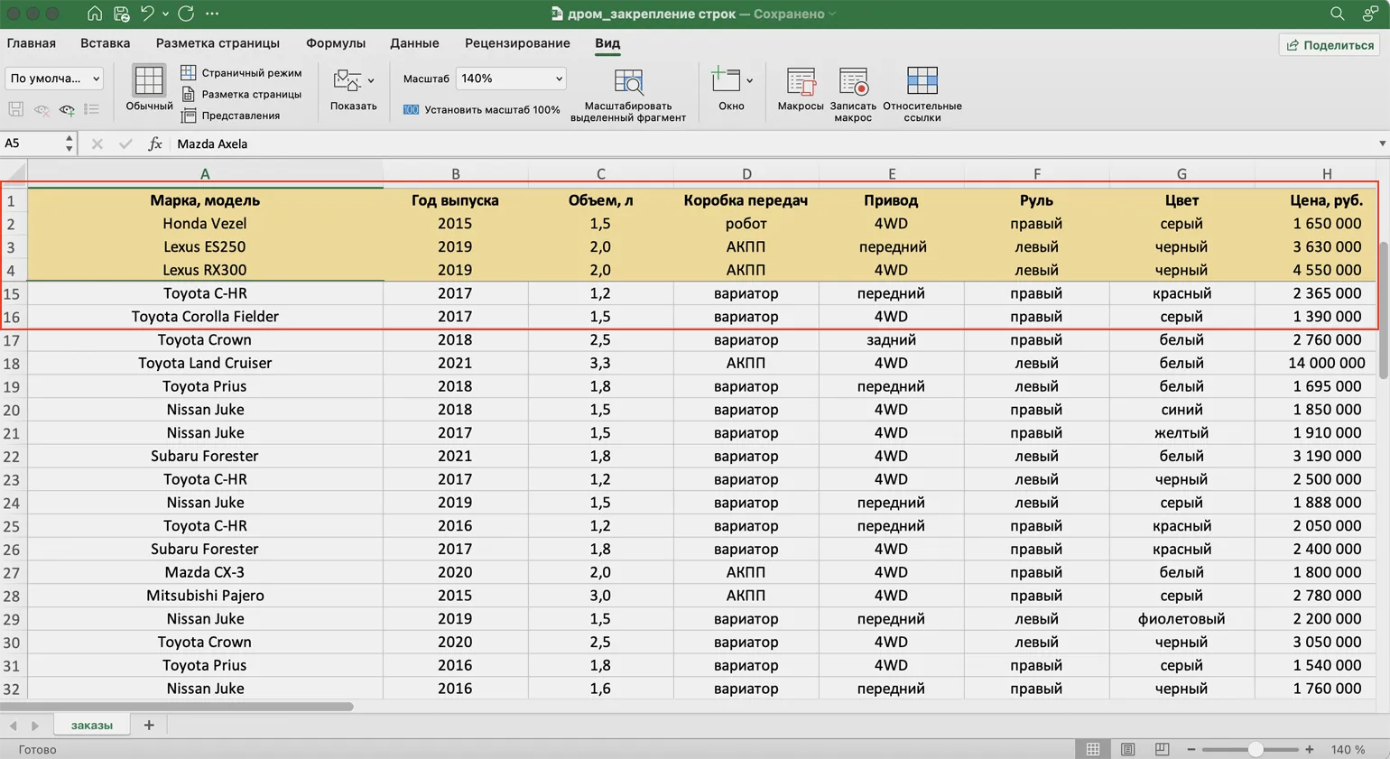
If you need to freeze not only the heading but also several lines of text, this is entirely possible. Let's start by highlighting the first three lines for ease of navigation and subsequent editing. This approach provides a more structured and understandable format for the information, which improves the user experience and facilitates better perception of the content.
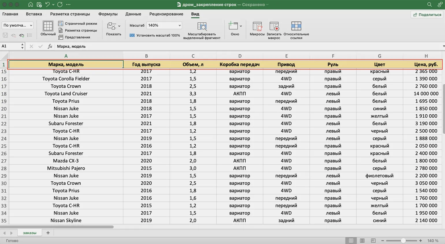
To freeze multiple rows in a table, first select the cell below the rows you want to freeze. In this case, it can be any cell in the fifth row.
Go to the "View" tab in your application, then click the "Window" button and select "Freeze Panes." This feature allows you to freeze multiple rows at once, making it easier to work with large tables and data. Freezing panes is useful for easily viewing headers and important data, ensuring efficient interaction with information as you work.
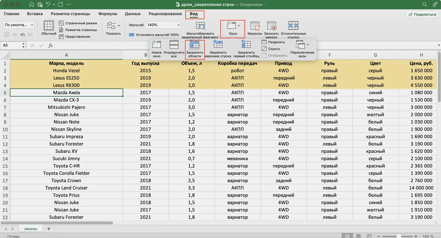
Now there's a border below the fourth table row, allowing frozen rows to remain visible while scrolling. This significantly simplifies table navigation and improves information comprehension, especially when working with large amounts of data. Users will be able to find the data they need faster without losing sight of important headings.
How to Freeze Columns in Excel
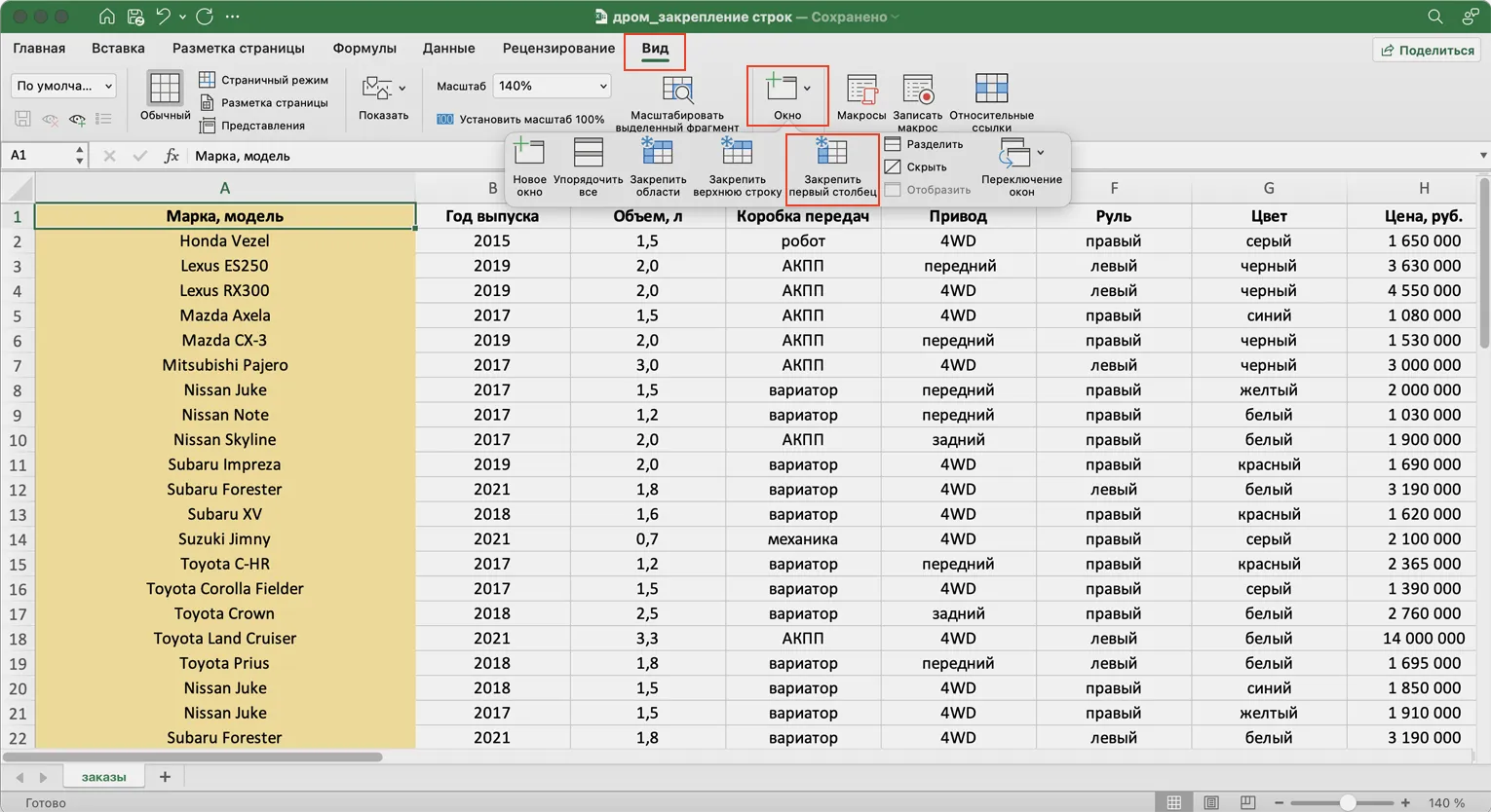
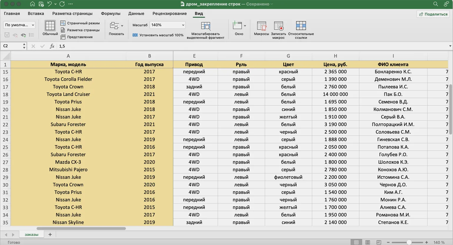
Freezing columns in Excel is an important feature that allows you to keep key information on the screen, even as you scroll through the spreadsheet. This feature is especially useful for working with large amounts of data when you need to constantly see headings or important categories of information. For example, the first column with the names of car makes and models, highlighted in yellow in the image, should always remain visible. This simplifies data analysis and increases the efficiency of working with tables in Excel.
- Select any cell in your table.
- Go to the "View" tab.
- Click the "Window" button and select the "Freeze First Column" option.
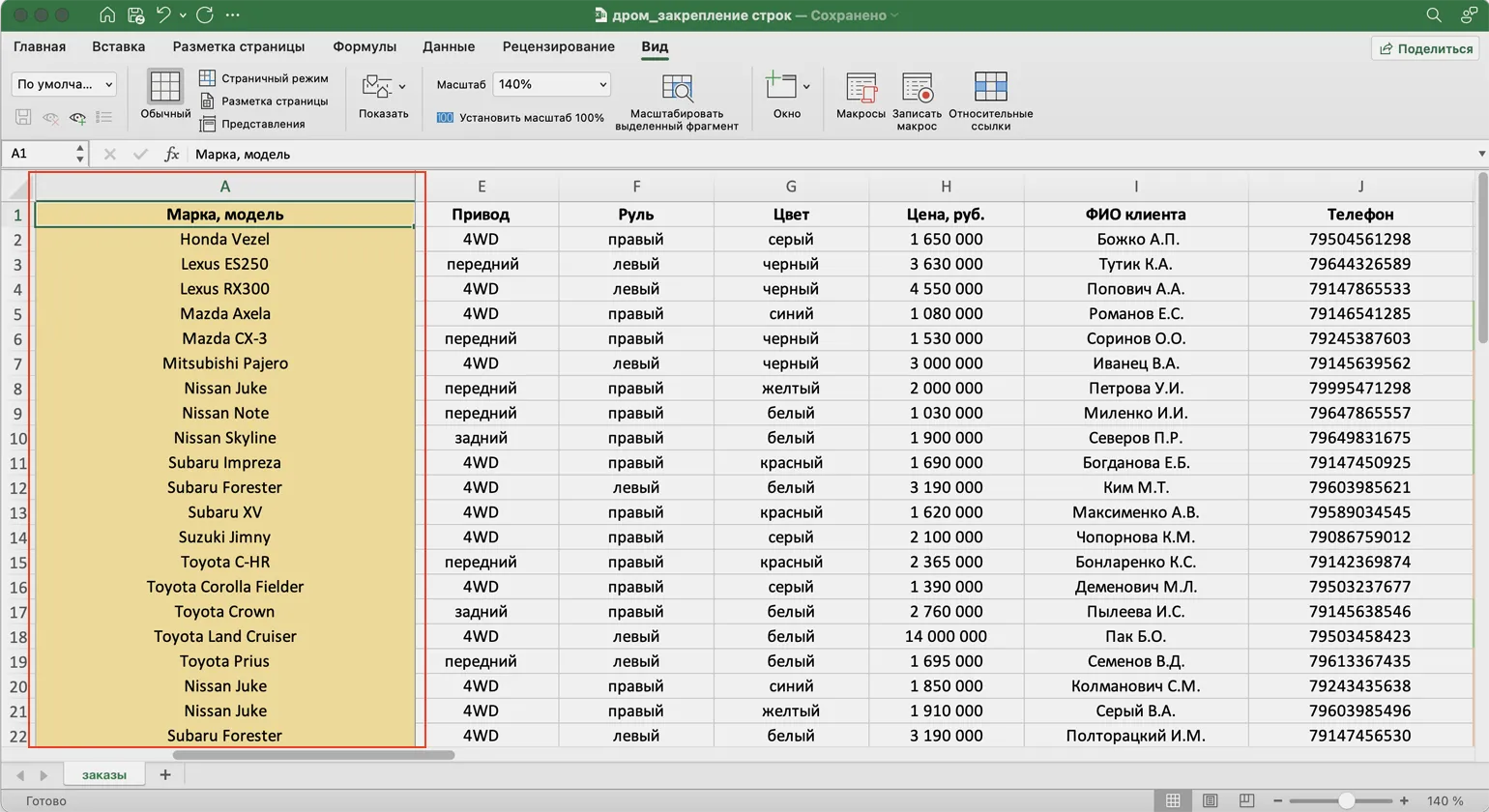
After completing these steps, a border will be added to the right of the first column. This will allow the make and model of cars to remain visible when scrolling horizontally, which will greatly simplify working with data and improve the perception of information.
If you need to freeze information from the first two columns for easier work, you can do so in just two simple steps. This will allow you to effectively organize your data and improve interaction with the table.
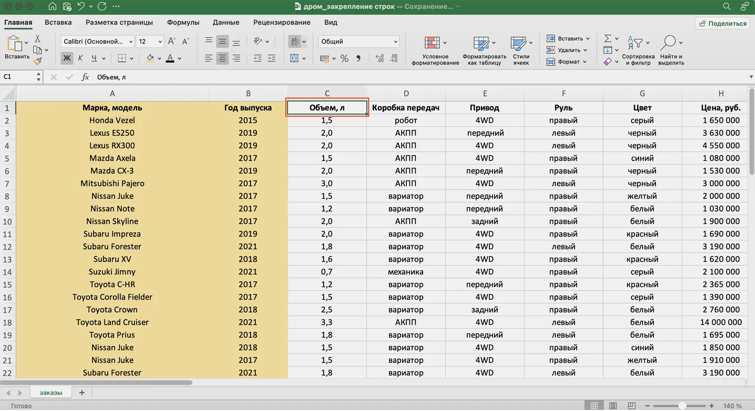
First, select the first cell in the column to the right of the columns you want to freeze. In this case, it's the cell in the first row of column C.
Go to the View tab, click the Window button, and select Freeze Panes. This will lock selected panes in the document, making it easy to edit and view data. Freezing panes helps improve navigation in long tables and allows you to focus on important data without losing sight of headings and key information.
After completing the specified actions, the border will be displayed to the right of the second column. Now, in any part of the table, you can easily view the makes and models of cars, as well as their year of production, which greatly simplifies working with data and increases the efficiency of information analysis.
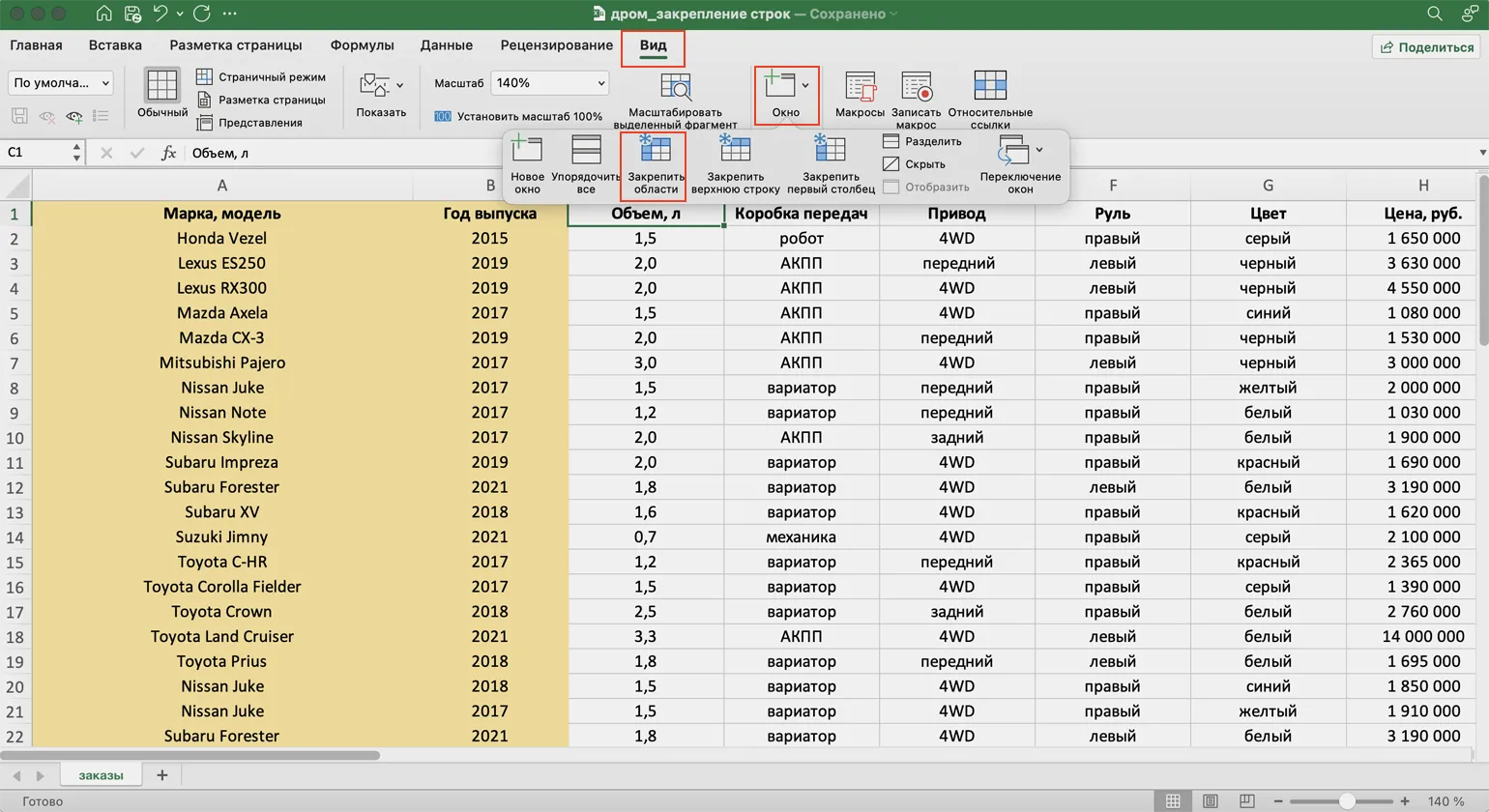
How to Freeze Rows and Columns in Excel
Working with large tables in Excel can be challenging, especially when you need to see headers and key information at all times. For example, perhaps you want the table header and the first two columns with car makes and years to remain on screen at all times. In this article, we'll take a detailed look at how to freeze the first row and the first two columns at the same time, which will greatly simplify your work with data in Excel. Freezing these elements will allow you to easily navigate the table without losing sight of important data.
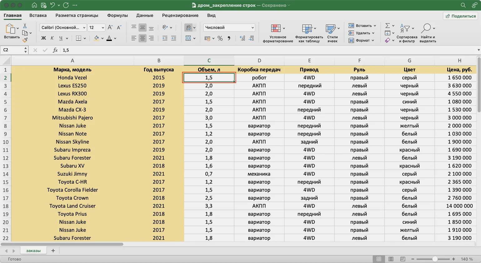
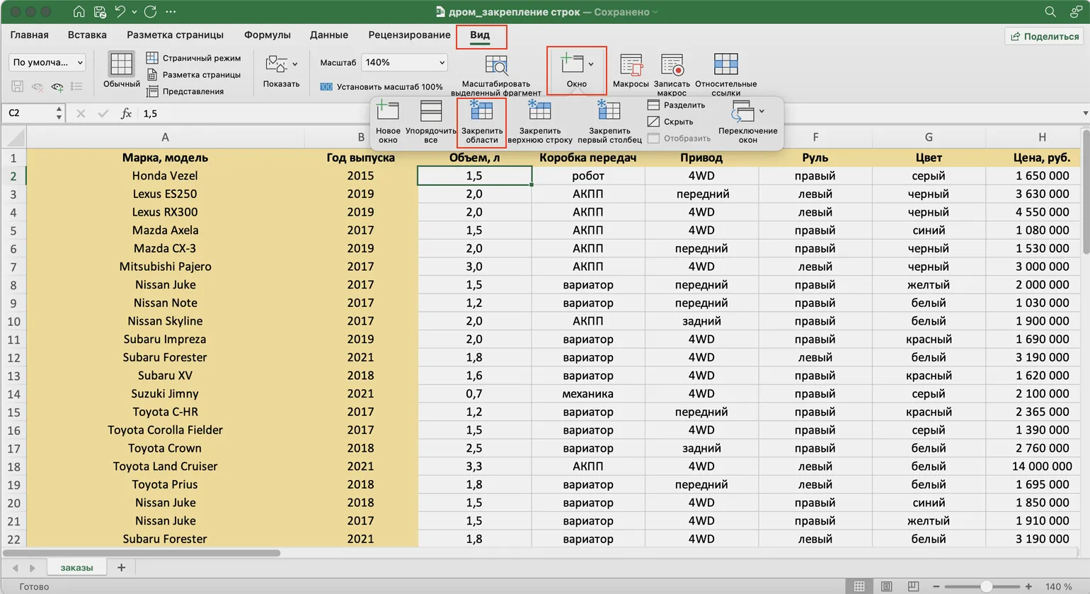
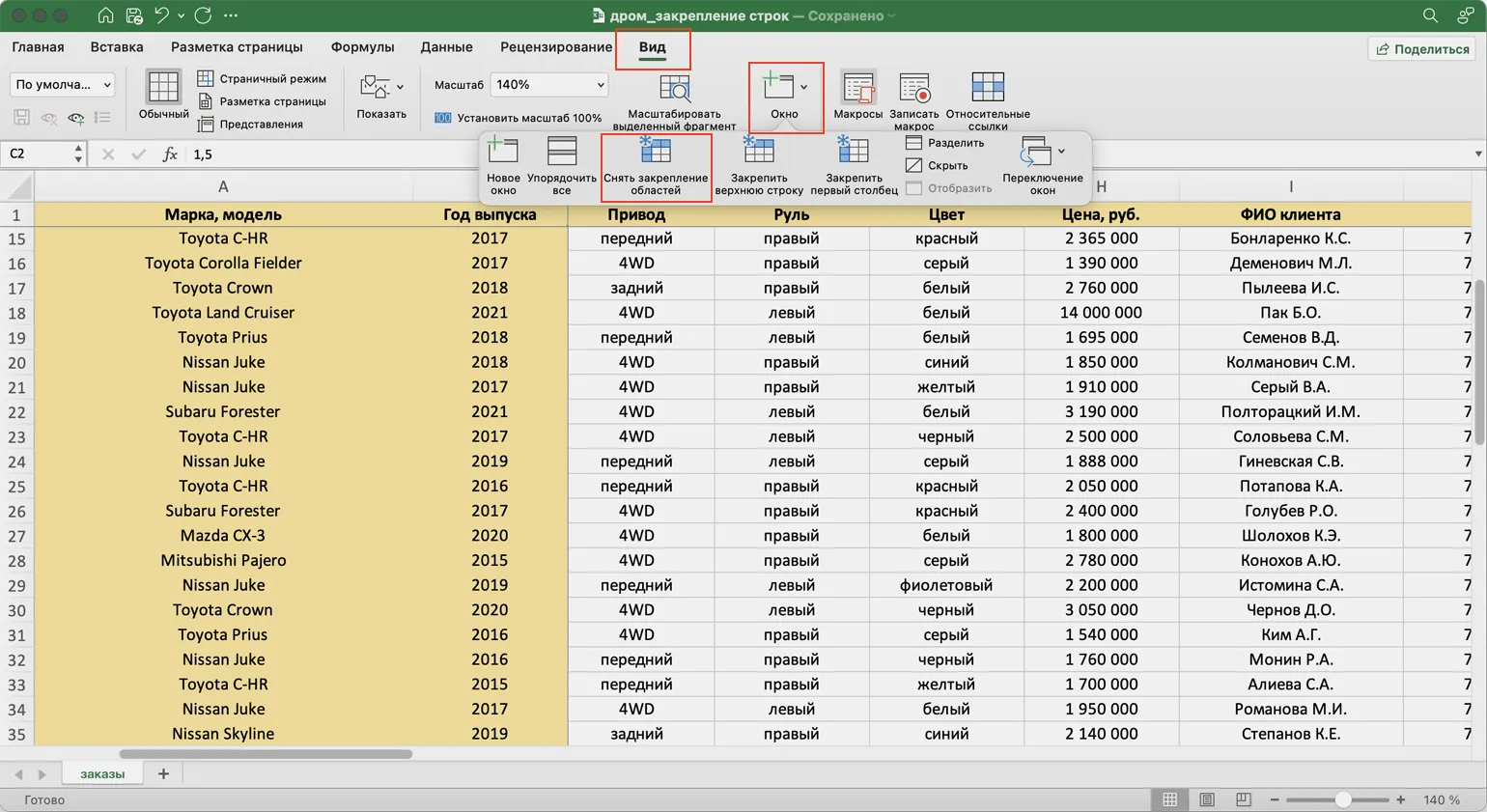
To freeze cell areas in a table, start by activating the cell located at the intersection of the rows and columns you want to keep visible. In this case, that's cell C2. This step is key, as it determines the area that will remain on screen while scrolling the table. Properly setting up frozen cells improves data perception and makes it easier to work with large tables.
Click the "View" tab in the top toolbar. Then click the "Window" button and select "Freeze Panes." This process will help Excel determine which data should remain visible on the screen, improving your workflow with large amounts of information.
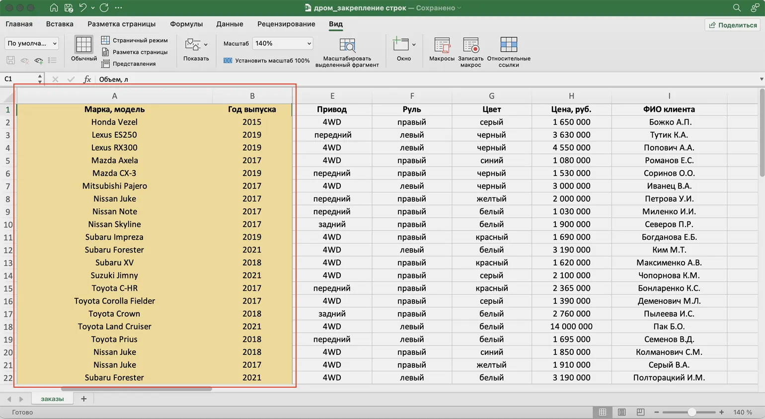
After completing these steps, you'll notice that the freeze borders appear to the right of the second column and below the first row. This means you can now scroll the table while keeping key headings and information about car makes, models, and production years visible. Freezing columns and rows makes it much easier to navigate your data, allowing you to quickly find the information you need.
How to Unfreeze Panes in Tables
To unlock frozen panes in tables, follow a few simple steps. Go to the "View" tab, then click the "Window" button and select "Unfreeze Panes." This action will return the table to the standard data view, which will allow you to easily view and edit all the information.
After completing these steps, all frozen areas of the table will be successfully unlocked. You can now edit the table in its original format. If necessary, you can also freeze other rows and columns to improve your data management experience.
Explore additional resources to help you develop your management and analytics skills. These resources offer valuable information and practical advice to help you grow professionally and improve your performance.
- Expert Interview: Who is a Business Analyst and What Do They Do?
- Ten Non-Obvious Mistakes Remote Team Leaders Make – Why Employees Leave
- A Deep Dive: What is Change Management in Companies?
- Manager's Dictionary: Understanding Key Management Terms
- Article: What Are Lencioni's Team Vices and How to Fight Them?
Excel and Google Sheets: From Beginner to PRO in 30 Days
Want to automate your work with spreadsheets? Learn how to master Excel and Google Sheets quickly and efficiently!
Learn more